Grounding System Modelling: From Steady-State to Transient

Delving into the complex behavior of grounding systems at high frequencies. Explore how impedance changes, transient responses arise, and effective modeling techniques are crucial for optimal performance.

Published on Monday, July 22, 2024600+ Views5min read

Grounding System Modelling: From Steady-State to Transient

Appropriate design of grounding systems is a key factor ensuring the proper operation of electrical networks in terms of human safety, component protection, insulation coordination and ElectroMagnetic Compatibility (EMC). The grounding system performance in both static (low frequency) and dynamic (high frequency) regimes is important. In the static regime, the aim of grounding systems design is to provide the desired grounding resistance, ground potential rise, touch and step voltages in normal operating condition and subsequent to short circuit currents [1] and [2]. The low frequency analysis of grounding systems can be done either by making use of empirical formulae or using numerical electromagnetic methods formulated in static regime. These methods, however, fail in providing accurate results at high frequencies when used for the calculation of lightning generated overvoltages, in particular for large grounding systems where the equipotential assumption for ground conductors is violated. Instead, high frequency analysis of grounding systems is usually carried out by making use of rigorous numerical electromagnetic methods. In high frequency regime, the aim of grounding system design is to control the lightning generated overvoltages and also to mitigate the voltage differences among different parts of the grounding system subject to lightning current. It is noted that transient voltage disturbances within grounding systems can reportedly lead to malfunction of small signal instrumentations by drifting the voltage reference point.

Lightning impulse currents are usually characterized by a wide frequency content from DC to several MHz over which the grounding system reveals different behavior at different frequency intervals. Hence, to obtain accurate lightning generated overvoltages, one should properly take into account the frequency dependence of grounding systems.

grounding electrodes

The concept of transient behavior of grounding systems can be adequately described by evaluating the low and high frequency behavior of simple grounding electrodes. As known, grounding systems at low frequency reveal a resistive behavior so that they can be reasonably modeled by their DC resistance. The basic electromagnetic assumption in the low frequency is to consider the grounding conductors equipotential (by ignoring the propagation delay) when excited by the short circuit current. Although, this assumption is violated when the size of ground electrode becomes comparable to the wavelength of the excitation current, it is still acceptable to model the grounding systems by their DC resistance at low frequencies. To this aim, various methods such as numerical electromagnetic methods with static or quasistatic assumptions [3], closed-form empirical expressions [4]. It is noted however that closed form expressions are only available for simple vertical and horizontal ground electrodes.

At high frequencies, however, the grounding system behavior is more complicated and cannot be accurately modeled unless rigorous electromagnetic solution methods are used. In fact, in many studies, it is intended to evaluate the performance of grounding systems over a wide frequency interval from DC to several MHz. In practice, the maximum frequency of interest is dictated by the type of the particular analysis and the nature of the source of disturbance. So far, grounding systems have been modeled by different methods such as circuit theory [5] -[6], transmission line theory [7]-[9], and full-wave approaches such as finite difference time-domain method (FDTD), finite element method (FEM) [10], and the method of moments (MoM) [11]-[16]. Circuit-based methods and transmission line theory are construed as quasi-static approaches, which generally fail in prediction of high frequency behavior of grounding systems. The three last methods (i.e., FDTD, FEM and MoM) can be categorized as full-wave or electromagnetic field approaches with the ability of accurate evaluation of the grounding systems performance over a wide frequency range.

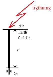
Fig. 1. Lightning striking a vertical ground electrode.

To better understand the high frequency behavior of grounding systems, let’s consider the case of a lightning strike to a vertical grounding electrode of length l= 3m and a circular cross-section of radius r=12.5 mm, buried in a soil with conductivity σ0 and relative permittivity $\eps_r$ , Fig. 1. A current of 1 A is injected into the grounding system at each frequency and the harmonic impedance Z(jω) of the grounding system is calculated as a function of frequency,

Z(j \omega) = \frac{V(j \omega)}{I(j \omega)}

where V(jω) and I(jω) are respectively the phasor of the electric potential at the feed point in reference to the remote earth and the phasor of the injected current [14]. The electric potential is calculated by integrating the electric field along a straight path starting from the electrode conductor surface to a point very far from the injection point in which the current approaches zero and could be physically considered as a voltage reference point. Fig. 3.2 shows the amplitude and the phase of the harmonic impedance of the vertical grounding electrode, computed using the FEM approach. The analysis is done for four different soil conductivities (i.e., σ0=0.01 S/m, 0.002 S/m, 0.001 S/m, 0.0005 S/m) having the same relative permittivity of $\eps_r$ =20. As it can be seen in these curves, the harmonic impedance, varies over the working frequency range. In the low frequency range, the magnitude of the harmonic impedance is equal to the static resistance (also called the DC resistance) while it takes different values for higher frequencies. This behavior of grounding electrodes is well known and has been thoroughly discussed (e.g., [14] and [16]). This is quite different from the static model of the grounding system which fails in providing accurate results at high frequencies when used for the calculation of the grounding system overvoltages. In another simulation case, the same vertical grounding electrode with a different length of l= 30m is analyzed. The amplitude and the phase of the harmonic impedance of this grounding electrode are shown in Fig. 2. Further examination on this figure reveals that the inductive or capacitive behavior of grounding electrodes is mainly determined by the soil electrical parameters as well as the length of the electrode. As it is seen in Fig. 3, at higher frequencies and for high conductive soils, the inductive behavior is dominant. It is quite different from the previous case in which the grounding electrode exhibits a capacitive behavior over the frequency range of interest This behavior complies with our expectation of capacitive behavior of grounding electrodes of small and moderate length buried in poor conductive soils with respect to long grounding electrodes [16]. The frequency at which the harmonic impedance deviates from the DC resistance and switches to either inductive or capacitive behavior is known as characteristic frequency.

Fig. 2. Harmonic impedance to ground for a vertical grounding rod of length l=3 m and circular cross-section of radius r=12.5 mm [14].

Fig. 3. Harmonic impedance to ground for a vertical grounding rod of length l=30 m and circular cross-section of radius r=12.5 mm [14].

Fig. 4. Frequency dependence behavior of grounding system impedance. Adapted from [17].

Fig. 4 shows typical frequency dependence behavior of grounding system impedance. In this figure the harmonic impedance |Z(jω)| is normalized by being divided to the low frequency resistance to earth Rg. From this figure and referring to circuit terms, the grounding system may behave as i) dominant capacitive circuit (|Z(jω)|/Rg < 1), ii) resistive circuit (|Z(jω)|/Rg = 1) or iii) inductive circuit (|Z(jω)|/Rg > 1). The impedance is nearly constant in the low frequency range while it shows a frequency dependent behavior at high frequencies. These two regions are distinguished by characteristic frequency Fc [17].

In grounding system design, resistive and capacitive behavior is more preferred since the HF impedance takes values equal or smaller than the LF resistance. The capacitive behavior is typical for short ground electrodes buried in highly resistive soils. Fig. 5 gives the regions of inductive and capacitive behavior of vertical and horizontal ground electrodes depending on the length, earth resistivity and discharge point [17]. Attention should be made to the DC resistance value when the goal is to decrease the HF value of the harmonic impedance by decreasing the length of electrode. In fact, it might not be practical choice since it might contradict with the intended values of the DC resistance as it usually requires longer electrodes.

Fig. 5. Behavior of ground electrodes depending on electrode length and soil resistivity. Adapted from [17]

Evaluation of transient behaviour of earth electrodes

Some parameters are usually defined to characterize transient behavior of grounding systems. Having calculated the harmonic impedance of grounding systems i.e., Z(jω), the time function of the voltage to earth (transient voltage) at the injection point v(t) can be readily calculated by applying the lightning current i(t),

v(t) = F^{-1} \{ Z(j \omega) \cdot F \{ i(t) \} \}

where F and F-1 denote Fourier and inverse Fourier transforms respectively.

The impulse impedance z0(t), is defined as the ratio of time domain voltage at the injection point to the injected current [17]:

Z_0(t) = \frac{V(t)}{i(t)}

Alternatively, the conventional impulse impedance Z could be used. This impedance is defined as the ratio of the maximum value of v(t) to the peak value of injected current i(t):

Z = \frac{\max[V(t)]}{\max[i(t)]} = \frac{V_{\max}}{I_{\max}}

The impulse efficiency is defined as the ratio between the conventional impedance and the low frequency resistance Rg, i.e., Impulse efficiency = Z / Rg.

It is worth mentioning that better impulse performance is associated with lower value of the impulse efficiency.

For a vertical grounding electrode subjected to a lightning subsequent return stroke current (Fig. 6), the impulse impedance vs. the electrode length is shown in Fig. 7 for different values of soil conductivity (i.e., σ0=0.01, 0.002, 0.001 S/m) having the same relative permittivity of $\eps_r$ . It is also seen that the longer the electrode the lower the impulse impedance. This reduction effect of the electrode length on the impulse impedance is, however, limited by the effective length of the electrode; a length beyond which the impulse impedance does not vary any more.

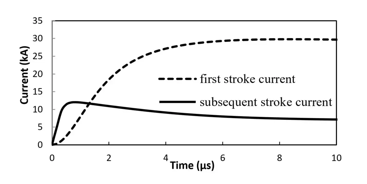
Fig. 6. Typical waveforms of lightning First and Subsequent return stroke currents

Fig. 7. Impulse impedance of a vertical grounding rod subjected to lightning subsequent return stroke shown in Fig. 3.6 [17]

It is noted that use of multiple ground electrodes specially close to the injection point improves the impulse efficiency of grounding systems. Horizontal rods are slightly less effective at power frequency in comparison to vertical rods, but have better impulse efficiency [17].

Fig. 8. An equally-spaced d1×d2 square grounding grid buried in depth h of a lossy soil. Adapted from [14]

Complex grounding systems

The complex grounding systems usually involve a combination of vertical and horizontal grounding electrodes and could be in the form of very large grounding grids. The transient performance of these systems is similarly evaluated by making use of rigorous electromagnetic methods. Generally speaking, these systems similar to the case of simple grounding electrodes reveal a frequency dependence behavior in particular at high frequencies. To better understand the behavior of complex grounding systems, we consider the case of a grounding grid buried in a single layer lossy soil, Fig.8. The grounding grid in this case is an equally-spaced d1×d2 square. The depth of the grid is h and the conductors are of radius r=12.5mm. The performance of the grounding grid is obtained while it is buried in a homogeneous single layer soil which is characterized by conductivities of σ0=0.01 S/m, 0.002 S/m, 0.001 S/m and a relative permittivity $\eps_r$ .

The magnitude and phase of the harmonic impedance of the grounding grid with h=0.5m, d1=2m and d2=3m are shown in Fig. 9. As it can be seen in this figure, the harmonic impedance takes different values over the working frequency interval showing either an inductive or capacitive behavior depending on the soil conductivity. Fig. 9 shows the voltage at the injection point for the same grounding systems for lightning first and subsequent return stroke currents of Fig.6.

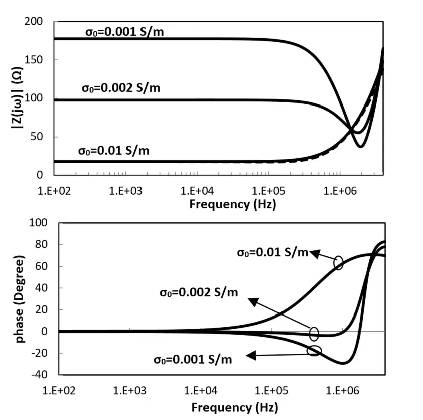
Fig. 9. Harmonic impedance of the grounding grid shown in Fig. 10, h=0.5m, d1=3m, d2=2m buried in a lossy soil.

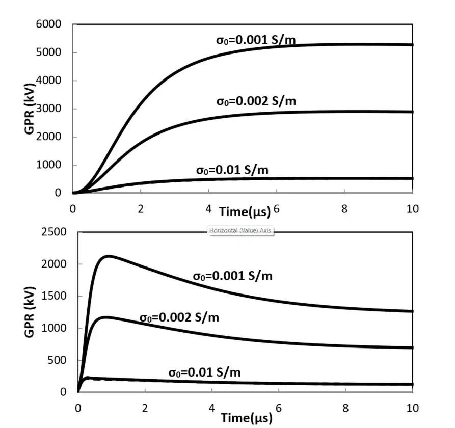
Fig. 10. GPR of the grounding grid shown in Fig. 9, h=0.5 m, d1=3m, d2=2m subjected to lightning first (up) and subsequent (down) strokes current.

Effect of frequency dependence of soil electrical parameters

The frequency dependence of soil conductivity and relative permittivity depends on a combination of factors such as dipolar molecules polarization, counter ion diffusion polarization (due to separation of cations and anions), interfacial (Maxwell-Wagner) polarization as well as various conduction and loss mechanisms, each acting on a specific frequency interval [19]-[23]. Owing to this fact, the soil conductivity and relative permittivity reveal a frequency-dependent behavior over the frequency range of interest. Therefore, using an accurate model of soil could help with acquiring a more precise analysis of grounding system transient behavior. One of the widely used models for modeling the frequency dependence of soil electrical parameters is the analytical formulae proposed by Longmire and Smith [19]. These equations read,

\rho_0 = 125 \cdot (\frac{p}{10})^{-0.54} (\Omega \cdot m), \quad \epsilon_{\infty} = 5

\rho(f) = (\rho_0^{-1} + 2 \pi \epsilon_0 \sum_{n=1}^{14} \frac{a_n (\frac{p}{10})^{1.28 \cdot 10^{n-1}} (\frac{f}{ (\frac{p}{10})^{1.28 \cdot 10^{n-1}}})^2}{1 + (\frac{f}{(\frac{p}{10})^{1.28 \cdot 10^{n-1}}})^2})^{-1}

\epsilon_r(f) = \epsilon_{\infty} + \sum_{n=1}^{14} \frac{a_n}{1 + (\frac{f}{(\frac{p}{10})^{1.28 \cdot 10^{n-1}}})^2}

where f is the frequency ranging from DC to 2 MHz, ρ(f) and εr(f) are respectively the soil resistivity and relative permittivity, ρ0 is the low-frequency resistivity, p is the water percentage of soil and an are coefficients presented in Table I [19].

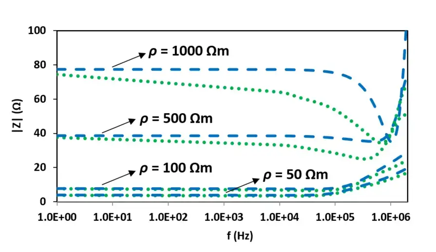
Harmonic impedances of the vertical rod for different soil resistivities. blue-dashed line: soil with constant electrical parameters, green-dotted line: soil with frequency-dependent electrical parameters.

Fig. 11. Harmonic impedances of the vertical rod for different soil resistivities. blue-dashed line: soil with constant electrical parameters, green-dotted line: soil with frequency-dependent electrical parameters.

Fig. 11 shows the amplitude of the harmonic impedance of the vertical grounding electrode, computed using the MoM approach presented in [24]. The impedance is calculated in frequency range of DC to 2 MHz for both soils with constant and frequency-dependent electrical parameters. Generally speaking, the frequency dependence of the soil electrical parameters for soils of high conductivity could be reasonably disregarded. Nevertheless, for the poorly conducting soils (conductivities around σ0<=0.002 S/m) the frequency dependence of the soil conductivity and relative permittivity needs to be taken into account to correctly simulate the performance of grounding systems. It should be also noted that the effect of the frequency dependence of soil electrical parameters can be particularly significant when grounding systems are subjected to subsequent return stroke currents. This effect is much more pronounced for long electrodes buried in highly resistive soils.

Fig. 12. Circuit representation of a vertical grounding rod based on the high frequency distributed parameters. Adapted from [32].

Equivalent circuits for high frequency modeling of vertical and horizontal ground electrodes

A distributed-parameter circuit can be used to adequately represent the harmonic impedance of the vertical and horizontal grounding rods [16] and [31]. In this approach the vertical grounding rod is divided into N fictitious segments and each segment of the rod is represented by an R-L-C section, Fig.12. For each segment the parameters are identical and defined as,

R_n = \frac{\rho N}{2 \pi l} (log \frac{4l}{r} - 1) \quad (\Omega)

C_n = \frac{2 \pi \epsilon l}{N} (log \frac{4l}{r} - 1) \quad (F)

L_n = \frac{\mu_0 l}{2 \pi N} (log \frac{2l}{r} - 1) \quad (H)

where, l is the length of the vertical rod and r is the radius. Rn, Ln and Cn are respectively the resistance, inductance and capacitance for each segment. $\rho$ is the soil resistivity (supposed to be homogeneous) in $\Omega$ m, $\mu$ o= 4 $\pi$ 10-7 H/m and $\eps$ is the soil permittivity (typical value : $\eps$ = 10 $\eps$ o with $\eps$ o = 8.85x10-12 F/m).

The vertical and horizontal ground electrodes can be modeled by their characteristic impedance and their propagation constant similar to the case of transmission lines. In doing so, Equations (3.7.a) and (3.7.bb) can be used for vertical rod [33] and [34]:

Z_c = \frac{A_1}{2 \pi} \sqrt{\frac{j \omega \mu_0 \rho}{(1 + j \omega \epsilon \rho)}}, \quad \gamma = \sqrt{j \omega \mu_0 (1/\rho + j \omega \epsilon)}

and for horizontal rod:

Z_c = \frac{A_2}{\pi} \sqrt{\frac{j \omega \mu_0 \rho}{2(1 + j \omega \epsilon \rho)}}, \quad \gamma = \sqrt{j \omega \mu_0 (1/\rho + j \omega \epsilon) / 2}

Therefore, in comparison to 50 / 60 Hz case, where grounding resistance can be simply computed for vertical and horizontal rod as:

R_g = \frac{\rho}{2 \pi \ell} A_1, \quad \text{and} \quad R_g = \frac{\rho}{\pi \ell} A_2,

Grounding impedance is complex and frequency dependent.

References

[1] IEEE Guide for Safety in AC Substation Grounding, IEEE Std. 80, January-2000.

[2] IEEE Recommended Practice for Grounding of Industrial and Commercial Power Systems (IEEE Green Book). IEEE Std 142 – 1991.

[3] Y. L. Chow and et al.,“ Surface voltages and resistance of grounding systems of grid and rods in two-layer earth by the rapid Galerkins moment method,” IEEE Trans. Power Del., vol. 12, pp. 179-185, Jan. 1997.

[4] Sunde, E. D. 1968. Earth Conduction Effects in Transmission Systems. Dover.

[5] A. F. Otero, J. Cidras, and J. L. Alamo, “Frequency-dependent grounding grid calculation by means of a conventional nodal analysis technology”, IEEE Transactions on Power Delivery, vol. no. 3, pp. 873-877, July 1999.

[6] B. Zhang, J. He, J. B. Lee, X. Cui, Z. Zhao, J. Zou, and S. H. Chang, “Numerical analysis of transient performance of grounding systems considering soil ionization by coupling moment method with circuit theory,” IEEE Transaction on Magnetics, vol. 41, no. 5, pp.1440-1443. MAY 2005.

[7] F. Menter and L. Grcev, “EMTP-based model for grounding system analysis,” IEEE Trans. Power Delivery, vol. 9, no. 4, pp. 1838-1849, Oct. 1994.

[8] L. Yaqing, M. Zitnik, and R. Thottappillil, “An improved transmission line model of grounding system,” IEEE Trans. Electromagn. Compat., vol. 43, no. 3, pp. 348-355, Aug. 2001.

[9] Y. Liu, N. Theethayi, and R. Thottappillil, “An engineering model for transient analysis of grounding grid under lightning strikes: Nonuniform transmission-line approach”, IEEE Transactions on Power Delivery, vol. no. 2, pp. 722-730, Apr. 2005.

[10] L. Qi, X. Cui, Z. Zhao, and H. Li, “Grounding performance analysis of the substation grounding grids by finite element method in frequency domain” IEEE Transactions on Magnetics, vol. 43, no. 4, April 2007.

[11] L. Grcev and F. Dawalibi, “An electromagnetic model for transients in grounding systems,” IEEE Trans. Power Delivery, vol. 5, no. 4, pp. 1773-1781, Nov. 1990.

[12] L. Grcev, “Computation of transient voltages near complex grounding systems caused by lightning currents,” in Proc. IEEE Int. Symp. Electromagn. Compat., 1992, pp. 393-400.

[13] F. Dawalibi and A. Selby, “Electromagnetic fields of energized conductors,” IEEE Trans. Power Delivery, vol. 8, no. 3, pp. 1275-1284, Jul. 1993.

[14] M. Akbari, K. Sheshyekani, and M. R. Alemi, “The effect of frequency dependence of soil electrical parameters on the lightning performance of grounding systems,” IEEE Transactions on Electromagnetic Compatibility, vol. 55, no. 4, pp. 739-746, Aug. 2013.

[15] L. Grcev, “Computer analysis of transient voltages in large grounding systems,” IEEE Trans. Power Delivery, vol. 11, no. 2, pp. 815-823, Apr. 1996.

[16] L. Grcev and M. Popov, “On high-frequency circuit equivalents of a vertical ground rod” IEEE Trans. Power Delivery, vol. 20, no. 2, pp. 1598-1603, Apr. 2005.

[17] CIGRE Working Group C4.4.02, “Protection of MV and LV Networks against Lightning. Part 1: Common Topics”, Paris, 2012.

[18] R. Alipio, S. Visacro, "Frequency Dependence of Soil Parameters: Effect on the Lightning Response of Grounding Electrodes", DOI: 10.1109/TEMC.2012.2210227.

[19] C. L. Longmire and K. S. Smith, “A universal impedance for soils,”Topical Report for Period July 1–September 30, Defense Nuclear Agency, Santa Barbara, California, 1975.

[20] J. H. Scott, “Electrical and magnetic properties of rock and soil,” U.S.Geol. Surv., Dep. of the Interior, Washington, D.C., 1966.

[21] B. D. Fuller, and S. H. Ward, “Linear system description of the electrical parameters of rocks”, IEEE Trans. Geosci. Electron., GE-8 no. 1, pp. 7– 18. Jan. 1970.

[22] R. L. Smith-Rose, “The electrical properties of soils for alternating currents at radiofrequencies,” Proc. Royal Society, vol. 140, no. 841A, pp. 359–377, 1933.

[23] A. C. S. de Lima, and C. Portela, “Inclusion of Frequency-Dependent Soil Parameters in Transmission-Line Modeling”, IEEE Trans. Power Del., vol. 22, no. 1, pp.492-499, Jan. 2007.

[24] M. R. Alemi and K. Sheshyekani, “Wide-band modeling of tower footing grounding system for the evaluation of lightning performance of transmission lines”, IEEE Transactions on Electromagnetic Compatibility, vol. 57, no. 6, pp. 1627-1636, Dec 2015.

[25] A.R. Hileman, “Insulation Coordination for Power Systems,” NewYork: Marcel Dekker, 1999.

[26] F. M. Gatta, A. Geri, S. Lauria, and M. Maccioni, “Generalized pi-circuit tower grounding model for direct lightning response simulation,” Electr. Pow. Syst. Res., vol. 116, pp. 330-337, July 2014.

[27] K. Sheshyekani, M. Akbari, B. Tabei, and R. Kazemi, “Wide-band modeling of large grounding systems to interface with electromagnetic transient solvers,” IEEE Trans. Power Del., vol. 29, no. 4, pp. 1868-1876, Aug. 2014.

[28] CIGRE Working Group 01 (Lightning) of Study Committee 33 (Overvoltages and Insulation Co-ordination), “Guide to procedure for estimating the lightning performance of transmission lines,” Document 63, Oct. 1991.

[29] P. Chowdhuri, J. G. Anderson, W. A. Chisholm, T. E. Field, M. Ishii, J. A. Martinez, M. B. Marz, J. McDaniel, T. R. McDermott, A. M. Mousa, T. Narita, D. K. Nichols, and T. A. Short, “Parameters of lightning strokes: a review,” IEEE Trans. Power Del., vol. 20, no. 1, pp. 346-358, Jan. 2005.

[30] F. H. Silveira, S. Visacro, A. De Conti, and C. R. de Mesquita, “Backflashovers of transmission lines due to subsequent lightning strokes,” IEEE Trans. Electromagn. Compat., vol. 54, no. 2, pp. 316-322, April 2012.

[31] C. T. Mata, M. I. Fernandez, V. A. Rakov, and M. A. Uman, “EMTP modeling of a triggered-lightning strike to the phase conductor of an overhead distribution line,” IEEE Trans. Power Delivery. vol. 15, no. 4, pp. 1175–1181, Oct. 2000.

[32] K. Sheshyekani, S.H. H. Sadeghi, R. Moini, F. Rachidi and M. Paolone, “Analysis of Transmission Lines with Arrester Termination, Considering the Frequency-Dependence of Grounding Systems”, IEEE Transactions on Electromagnetic Compatibility, vol. 51, no. 4, pp. 986-994, Nov. 2009.

[33] S. Ramo, J. R. Whinnery, and T. van Duzer, Fields and waves in communication electronics, 3 ed. New York: Wiley, 1994.

[34] L. Grcev and V. Arnautovski, "Comparison between simulation and measurement of frequency dependent and transient characteristics of power transmission line grounding," presented at 24th International Conference on Lightning Protection (ICLP'98), Birmingham, U.K., 1998