
Large solar flares and their associated coronal mass ejections (CME) are intense solar activities which under certain circumstances can cause disturbances in the near-Earth space environment [1]. The CMEs contain up to 10 billion tons of plasma material whose travel time from the sun to Earth is about two days (but with widely varying transit times) [2]. The CME’s solar wind plasma can interact with the magnetosphere causing rapid changes in the distribution of Earth’s magnetic field, a form of space weather which is referred to as Geomagnetic Storm (GMS) (see Figure 1). These phenomenon can occur during any season and are somewhat independent of the usual 11- or 12-year sunspot cycle [3].
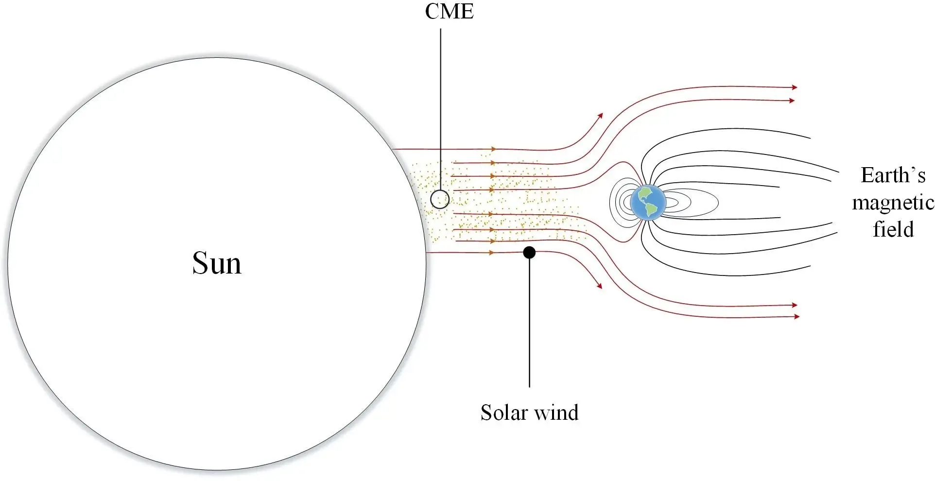
Figure 1: Effect of solar wind on earth’s magnetic field
The CME is regularly observed by the Solar and Heliospheric Observatory (SOHO), a spacecraft launched in 1995 and located in an orbit between Earth and the sun. Figure 2 shows the number of CME events recorded by SOHO over a period of several years (some data for late 1998 and early 1999 are missing).
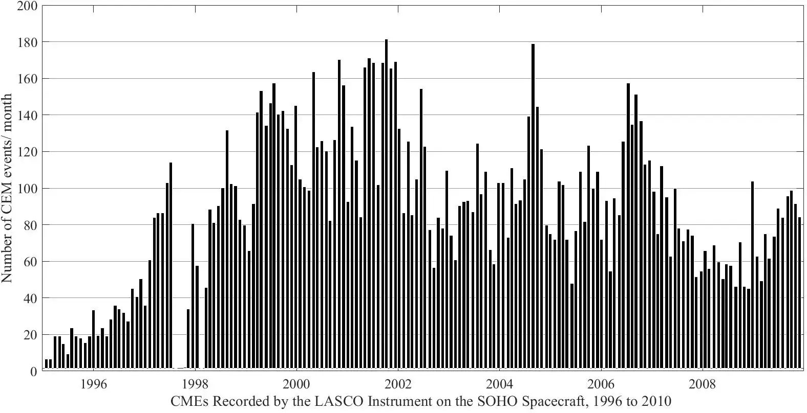
Figure 2: CMEs recorded by the LASCO instrument on the SOHO spacecraft, 1996 to 2010, adapted from [3]
The GMSs are random in terms of severity and timing. Richard Carrington, an English astronomer, has observed and recorded the event that occurred in 1859 from its outset on the surface of the sun. That storm, known as the Carrington Event, is generally acknowledged to be the largest in recorded history so far [4]. The space observations of celestial events has been performed during a period when power transmission and distribution systems did not exist, which makes direct comparisons with modern systems impossible. The Carrington Event, however, disrupted the telegraph system and resulted in fires in some telegraph offices. GMS produces impulsive disturbance of geomagnetic field over wide geographic regions which, in turn, induces currents (called geomagnetically-induced currents or GIC) on long transmission lines [5], [2]. Because of the size of the cross-sectional area of the single-turn loop represented by the power transmission line and the ground return path, the GIC could be quite large ( in the order of 100 amps or even more).
Proper evaluation of GIC and its effect on power systems requires modeling of a large-scale system accommodating long transmission lines in the order of hundreds of kilometers where a realistic 3-D structure of the propagation terrain must be considered.
Geomagnetic Storms and Their Adverse Effects
GMS electromagnetic fields (GS-EMFs) are characterized by an ultra-low frequency content (from 0.0001 Hz to 1 Hz) and can interact with power systems, resulting in significant low-frequency GIC on long transmission lines, see Figure 3. The adverse effects of GICs on the operation of bulk power systems are, but not limited to: half-cycle saturation in power transformers, harmonics, and increased reactive power demand and transformer spot heat [6]. These can ultimately result in transformer damage, voltage sags, relay malfunctioning, and system instability [7–9]. The effects of CMEs on power systems are detected every few years. These effects were observed in 1979, 1982, 1986, 1989, 1992, 1994, 1998, 2000, 2001, 2003, and 2005.
Large-scale blackouts happen less frequently but are a definitive risk. Severe CME events occurred in 1859 (disrupting the telegraph system), 1921, and 1989, when U.S. and Canadian utilities lost power transmission capabilities over wide areas. Recent studies reveal that GMDs do not only happen in high latitudes. In fact, the problems caused by GICs have also been reported in middle and low latitudes [10], [11], such as South Africa, Brazil, and China.
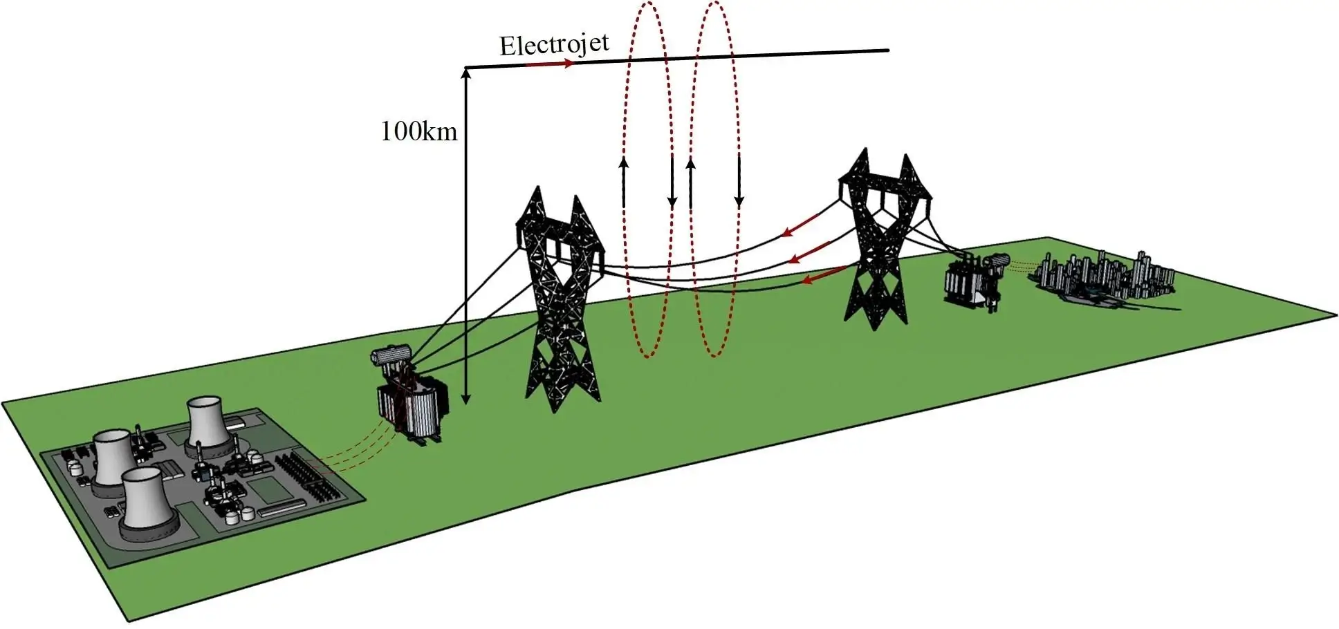
Figure 3: Geomagnetic storm modeled by an Electrojet and its associated GIC on overhead transmission lines.
Three major GMD events are shown in Table 1. The Hydro-Quebec blackout in 1989, which is attributed to a GMS, affected Canadian and U.S. power systems causing a major power outage due to cascading tripping of protection relays. Millions of people for several hours did not have access to electricity [12]. In 2003, the South Swedish power grid was affected by a large GMS which resulted in a GIC of 330 amperes, approximately. Subsequent to the flow of this GIC, a 130 kV transmission line has been knocked down. The consequent blackout lasted for an hour and left about 50,000 customers without electricity [13]. The GMS in 2015 was the largest in more than 15 years and is popularly known as the St. Patrick’s Day storm. During the intense period of the storm, global positioning system (GPS) receivers have been affected. These events initiated an extensive research on GMD effects on power systems.
Table 1: Major GMSs and their adverse effects
| Past Event | Year | Effect |
|---|---|---|
| March 1989 GMS | 1989 | Cascading tripping of Hydro-Quebec protection relays which resulted in a blackout that affected millions of consumers. |
| The Halloween Solar Storm | 2003 | GIC with a magnitude of 330 A led to a large-scale blackout by disconnecting a 130 kV transmission line. |
| St. Patrick’s Day storm | 2015 | Largest storm in more than 15 years. Planetary Index (Kp) reached 8 out of 9. GPS receivers signals were impaired. |
GIC Measurement and Monitoring
To measure GIC in a given power system, Hall effect sensors, as it is shown in Figure 4, are usually installed on the neutral conductor of the selected transformer where, with proper filtering and conditioning, the quasi-DC currents flowing through the transformer winding to ground are monitored [24].
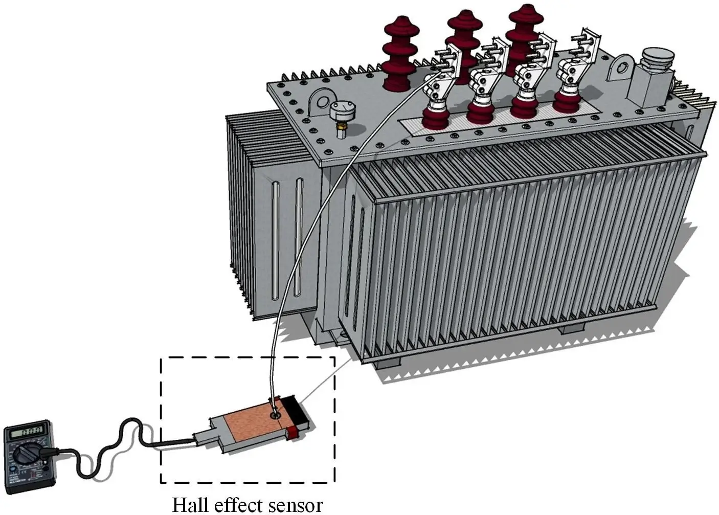
Figure 4: Hall Effect sensor installed on neutral point of a transformer to measure the GIC
The GIC monitoring can be alternatively done by measuring the capacitor bank and shunt reactor neutral current [25]. The Sunburst system, which uses this technique, was developed by the Energy Policy Research Institute (EPRI) and has been in use in the United States since 2004 (mainly in the north-east), Manitoba (on a feeder supplying Minnesota) [26], and in England and Wales [27]. The Minnesota power system also uses a direct DC current measurement mounted on a phase conductor of a 500 kV transmission line [25].
The major downside of this real-time monitoring technique is inability to provide the necessary warning in order to take remedial actions to protect the power system against GIC [26]. Almost all real-time monitoring techniques suffer from this drawback. The transformer neutral current monitoring can be practically performed for a few selected neutrals. Hence, to determine the GIC on all transmission lines, assumptions must be made about the geoelectric field [28]. Geo-electric fields generated by geomagnetic disturbances electromagnetic fields refer to the electric fields that are generated as a result of fluctuations in the Earth’s magnetic field. These fluctuations can be caused by geomagnetic storms, which are disturbances in the Earth’s magnetic field caused by charged particles from the Sun. These charged particles can interact with the Earth’s magnetic field, causing it to fluctuate, and induce electric currents in the Earth’s conductive layer. These induced electric currents can generate geo-electric fields at the Earth’s surface, which can be measured and used to study the Earth’s electrical conductivity and subsurface structure. The relationship between geomagnetic disturbances and geo-electric fields is complex and depends on various factors, including the conductivity of the Earth’s subsurface and the intensity of the geomagnetic storm. Understanding this relationship is important for a variety of applications, including predicting the effects of space weather on technology systems, such as satellites and power grids, as well as for improving our understanding of the Earth’s interior.
Transformer neutral currents are also used to trigger events such as dispatch alarms and fault recorders to facilitate management and analysis of GIC incidents [28]. The quantification of the GIC effect is carried out by monitoring system data and parameters including system voltages and reactive power consumption, as well as transformer tank temperature, transformer oil gassing, and transformer noise and vibration [28].
Researchers and utility companies are interested to better understand the GS-EMFs at ground surface in order to better understand GIC. Several methodologies and technologies have been developed in this regard [29]. Magnetic sensor, also known as a magnetometer, measures magnetic induction (magnetic field intensity), is used to measure and record magnetic field data initiated from GS-EMFs [28, 29]. As an alternative to magnetic field measurement, some have used grounded or isolated dipoles to measure electric fields [29].
Prediction of GIC
Real-time measurements keep record of GIC flowing through the system. This is useful for understanding the system status and for post-event analyses, although it provides limited assurance to system operators that a system will survive a GIC event [28, 29]. If reasonably accurate GIC predictions cannot be made, the only option is to react to every GIC that may potentially occur. Despite being conservative, by adopting this approach, utility and transmission system owners can be incurred due to unnecessary generation reduction and redistribution [30].
A simple approach is to perform GIC forecast based on an empirical equation which relates the observed (measured) time-derivative of the magnetic field dB , at a given site for every three hours (ap index) and the GICs that can flow into the power grid through earthing points at substations [31]. Similarly, the daily measurement of the time-derivative dB is represented in the Ap index which can also be used for the GIC prediction [44]. Many organizations use this method to plan activities that are dependent on the state of the Earth’s magnetic field. In terms of accuracy, such forecasts are not very accurate, accounting for only 29 percent of the variance in Ap. To overcome this problem, forecasters use properties of Ap and events on the Sun (i.e., solar flares, coronal mass ejections, and coronal holes) to predict Ap for the following day. The most prominent ones are persistence, 27-day recurrence, semiannual variation, as well as modulation of the solar cycle [32].
The main shortcoming of the above-mentioned prediction methods is that subsequent to power system topology changes, a new set of empirical data must be collected which makes these methods inflexible. A more sophisticated modeling technique relies on the prediction of the so-called auroral electrojet (ionospheric current) from which the magnetic field variations dB/dt are obtained. Hence, using Faraday’s law, the ground-surface electric potential V reads,
The geo-electric field can then be calculated from the ground-surface electric potential. Subsequently, different approaches such as circuit approach [33] can be adopted to obtain GIC from the associated geo-electric field. This calculation despite its simplicity relies on the availability of the earth conductivity model [34–36] which is not easy to obtain.
A more computationally efficient method to predict GIC is based on the measured or calculated Earth surface impedance Z (representing the Earth’s response). In this method the geo-electric field (Ey) is obtained from the horizontal magnetic field (Bx) [35, 36] as follows;
with µ0 being the magnetic permeability of free space. This approach, however, disregards the impact of conductive networks because of their larger grounding resistance as compared to the Earth surface impedance.
Geomagnetic Disturbance Modelling
To calculate the GIC for a given power system, the GS-EMFs at the ground surface should first be calculated. The majority of previous studies have used an auroral electrojet as the GS-EMF source [37–41]. Such a choice is reasonable, because at high latitudes, where the most significant geomagnetic effects are observed, geomagnetic disturbances are principally due to an auroral electrojet current system, which contains an intense east-west current (the electrojet) in the ionosphere [40]. To date, different analytical [38] and numerical methods [41] have been adopted for the calculation of GS-EMFs. In [51], the complex image method (CIM) [37] was used to compute GS-EMFs considering both single-layer and horizontally stratified multilayer grounds. The CIM demonstrated excellent accuracy for the case of horizontally stratified multilayer ground [38]. However, this method is not applicable to complex ground structures such as vertically or horizontally-vertically stratified ground. Furthermore, for particular cases (long TLs), the realistic 3-D structure of the propagation terrain must be taken into account, which is beyond the capability of classical 1-D approaches [38]. It is also worth noting that the classical 1-D method calculates the electromagnetic field in the absence of transmission line system, which reduces its accuracy. More recently, the effects of mixed multilayer ground on the electro-magnetic fields (EMFs) generated by an electrojet were evaluated by a 2-D finite element method (FEM) [41]. However, this method becomes computationally expensive for accurate 3-D modelling of large-scale propagation terrains.